


It is a spreadsheet program developed by Microsoft. Excel organizes data in columns and rows and allows you to do mathematical functions. It runs on Windows, macOS, Android and iOS.
The first version was released in 1985 and has gone through several changes over the years. However, the main functionality mostly remains the same.
Excel is typically used for:
- Analysis
- Data entry
- Data management
- Accounting
- Budgeting
- Data analysis
- Visuals and graphs
- Programming
- Financial modeling
- And much, much more!
Why Use Excel?
Get Started
This tutorial will teach you the basics of Excel.
It is not necessary to have any prior experience with spreadsheet programs or programming.
Office 365
The easiest way to get started with Excel, is to use Office 365.
Office 365 does not require downloading and installation of the program. It simply runs in your browser.
In our tutorial we will use Office 365, which can be accessed from www.office.com.
Install
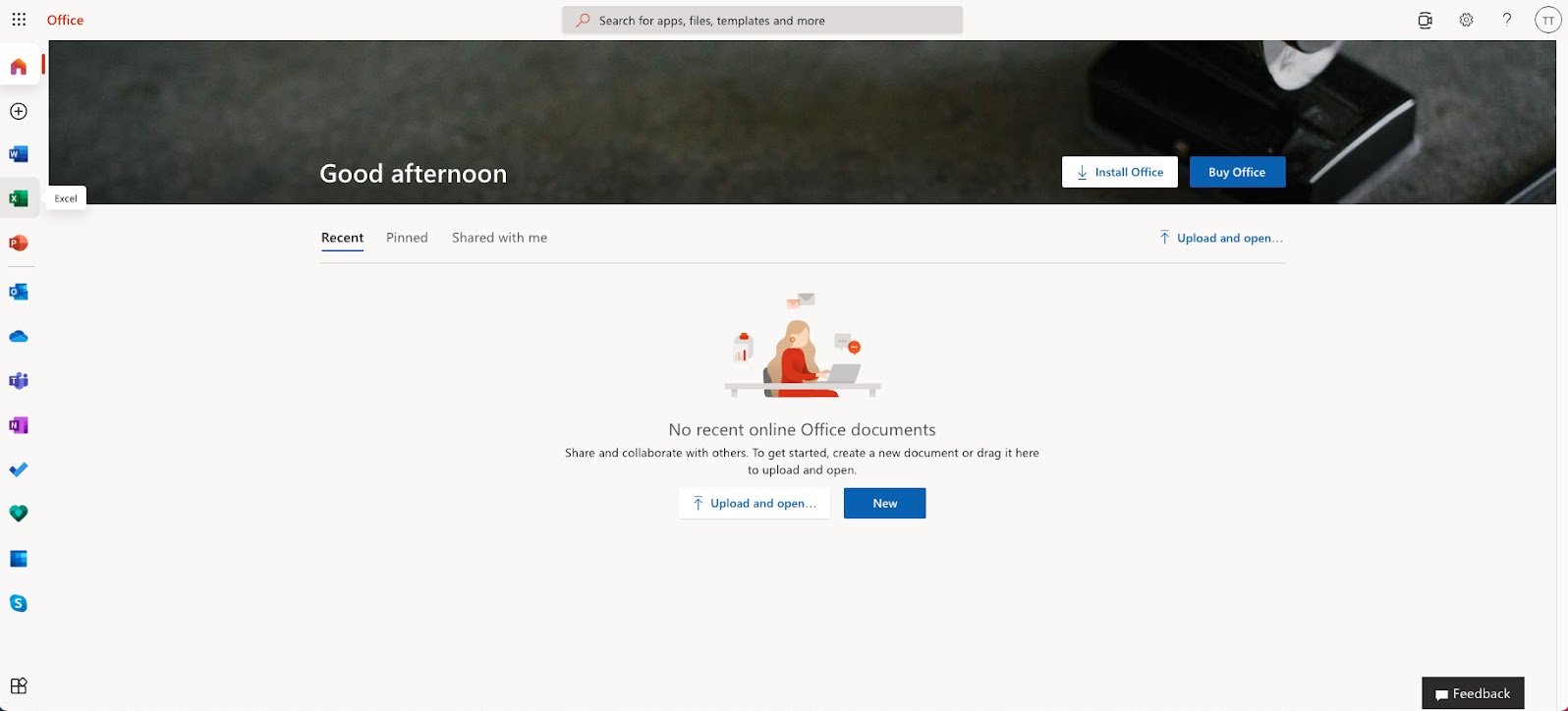
Once you have successfully logged into Office through www.office.com, click on the Excel icon on the left side to enter the application:
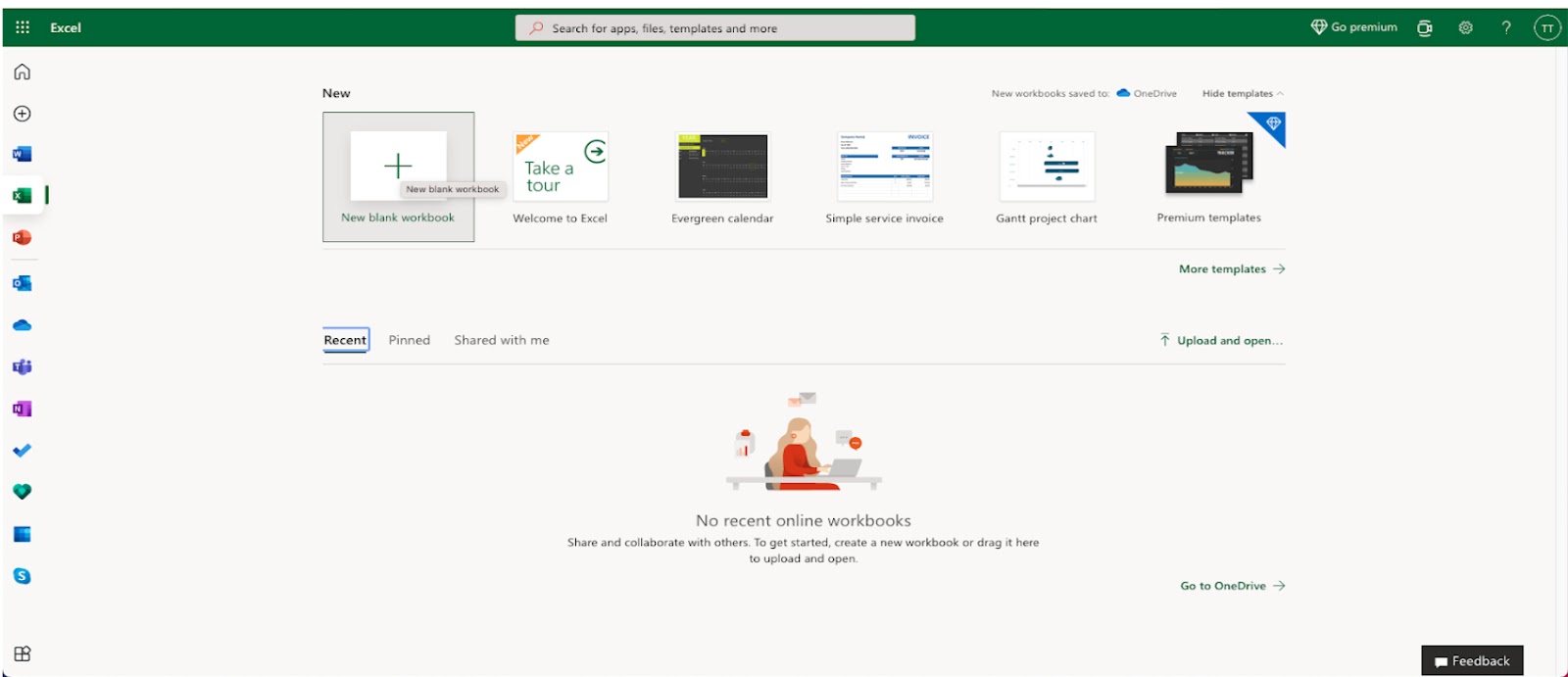
After entering the Excel application, click on the New blank workbook button to get started with a new workbook.
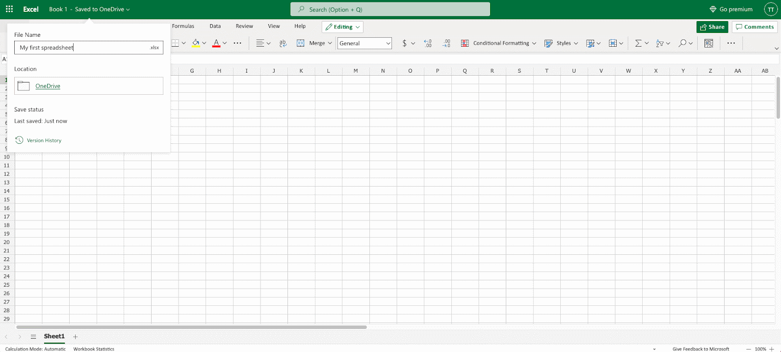
Enter a name for your workbook, and hit the enter button:
The Excel view has columns and rows, similar to a squared math exercise book.
Do not worry if the functionality looks overwhelming at first. You will get comfortable as you learn more in the chapters to come.
For now focus on the rows, columns, and the cells.
Ok. Let's make a function!
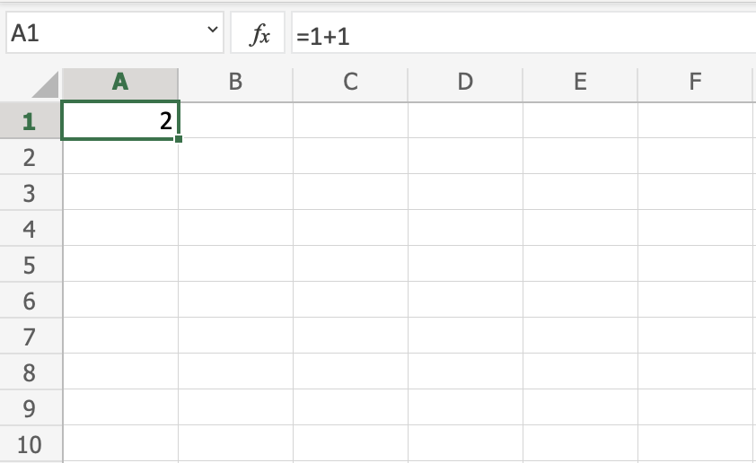
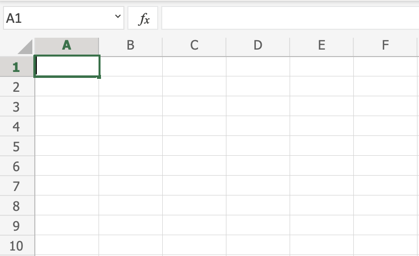
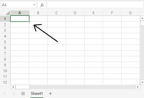
- First, double click the cell
A1, the one that is marked with the green rectangle in the picture. - Second, type
=1+1. - Third, hit the enter button:
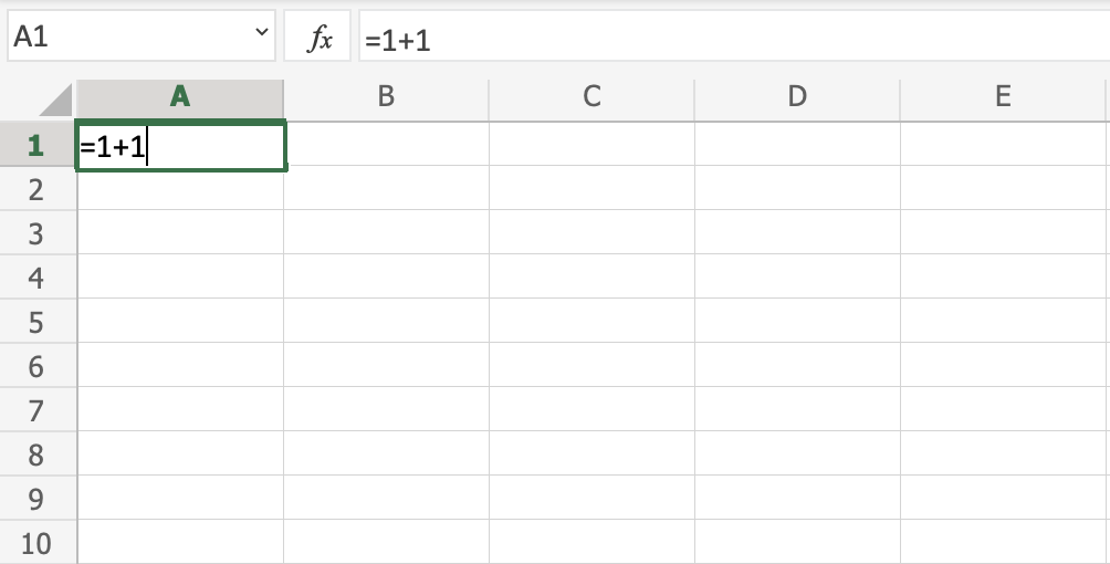
Congratulations! You have typed your first function, 1+1=2
Overview
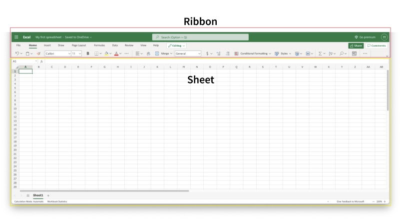
This chapter is about giving you an overview of Excel. Excel's structure is made of two pieces, the Ribbon and the Sheet.
Have a look at the picture below. The Ribbon is marked with a red rectangle and the Sheet is marked with a yellow rectangle:
First, let's start with explaining the Ribbon.
The Ribbon explained
The Ribbon provides shortcuts to Excel commands. A command is an action that allows you to make something happen. This can for example be to: insert a table, change the font size, or to change the color of a cell.
The Ribbon may look crowded and hard to understand at first. Don't be scared, It will become easier to navigate and use as you learn more. Most of the time we tend to use the same functionalities over again.
The Ribbon is made up by the App launcher, Tabs, Groups and Commands. In this section we will explain the different parts of the Ribbon.
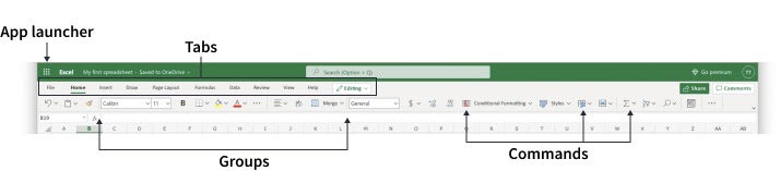
App launcher
The App launcher icon has nine dots and is called the Office 365 navigation bar. It allows you to access the different parts of the Office 365 suite, such as Word, PowerPoint and Outlook. App launcher can be used to switch seamlessly between the Office 365 applications.
Tabs
The tab is a menu with sub divisions sorted into groups. The tabs allow users to quickly navigate between options of menus which display different groups of functionality.
Groups
The groups are sets of related commands. The groups are separated by the thin vertical line break.
Commands
The commands are the buttons that you use to do actions.
Now, let's have a look at the Sheet. Soon you will be able to understand the relationship between the Ribbon and the Sheet, and you can make things happen.
The Sheet explained
The Sheet is a set of rows and columns. It forms the same pattern as we have in math exercise books, the rectangle boxes formed by the pattern are called cells.
Values can be typed to cells.
Values can be both numbers and letters:
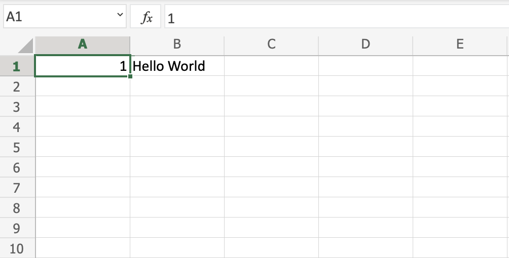
Each cell has its unique reference, which is its coordinates, this is where the columns and rows intersect.
Let's break this up and explain by an example
Have a look at the picture below. Hello world was typed in cell C4. The reference can be found by clicking on the relevant cell and seeing the reference in the Name Box to the left, which tells you that the cell's reference is C4.
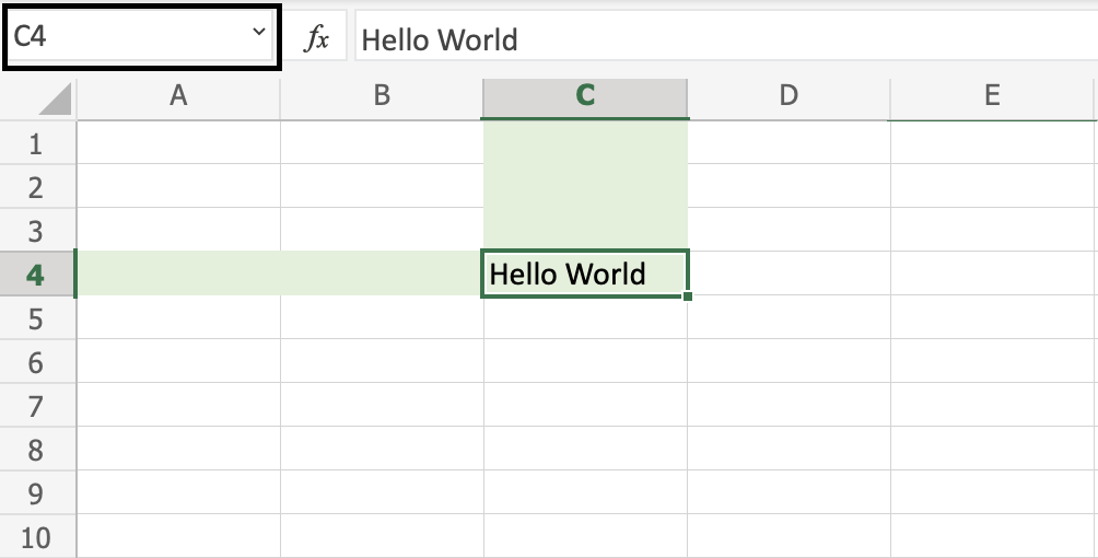
Another way to find the reference is to first find the column, in this case C, then map that towards the row, in this case 4, which gives us the reference of C4.
Multiple Sheets
You start with one Sheet by default when you create a new workbook. You can have many sheets in a workbook. New sheets can be added and removed. Sheets can be named to making it easier to work with data sets.
Are you up for the challenge? Let's create two new sheets and give them useful names.
First, click the plus icon, shown in the picture below, create two new sheets:
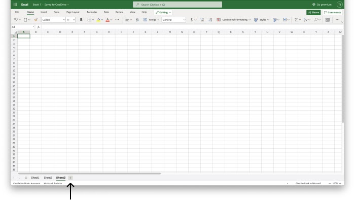
Tip: You can use the hotkey Shift + F11 to create new sheets. Try it!
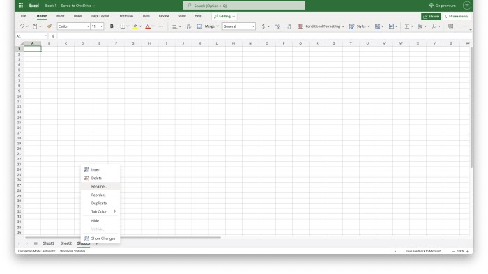
Second, right click with your mouse on the relevant sheet and click rename:
Third, enter useful names for the three sheets:
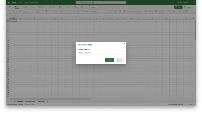
In this example we used the names Data Visualization, Data Structure and Raw Data. This is a typical structure when you are working with data.
Good job! You have now created your first workbook with three named sheets!
Chapter Summary
The workbook has two main components: the Ribbon and the Sheet.
The Ribbon is used to navigate and access commands.
The Sheet is made up of columns and rows, which make cells.
Each cell has its unique reference. You can add new sheets to your workbook and name them.
In the next chapters you will learn more about the sheet, formulas, ranges and functions.
Syntax
A formula in Excel is used to do mathematical calculations. Formulas always start with the equal sign = typed in the cell, followed by your calculation.
Note: You claim the cell by selecting it and typing the equal sign (=)
Creating formulas, step by step
- Select a cell
- Type the equal sign (=)
- Select a cell or type value
- Enter an arithmetic operator
- Select another cell or type value
- Press enter
For example =1+1 is the formula to calculate 1+1=2
Note: The value of a cell is communicated by reference(value) for example A1(2)
Using Formulas with Cells
You can type values to cells and use them in your formulas.
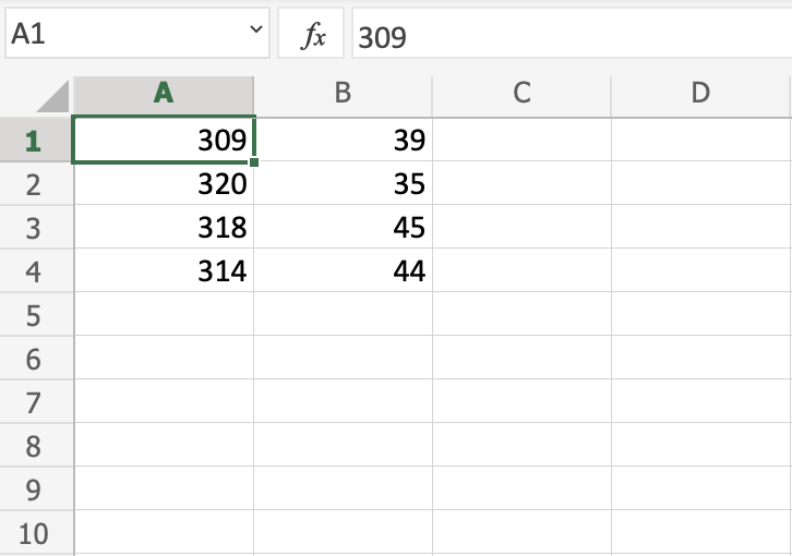
Lets type some dummy values to get started. Double click the cells to type values into them. Go ahead and type:
A1(309)A2(320)B1(39)B2(35)
Compare with the picture shown below:
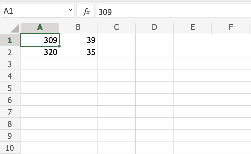
Note: Type values by selecting a cell, claim it by entering the equal sign (=) and then type your value. For example =309.
Well done! You have successfully typed values to cells and now we can use them to create formulas.
Here is how to do it, step by step.
- Select the cell
C1 - Type the equal sign (
=) - Left click on
A1, the cell that has the(309)value - Type the minus sign (
-) - Left click on
B2, the cell that has the(35)value - Hit enter
Tip: The formula can be typed directly without clicking the cells. The typed formula would be the same as the value in C1 (=A1-B2).
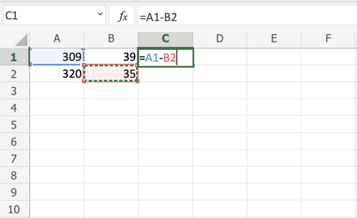
The result after hitting the enter button is C1(274). Did you make it?
Another Example
Let's try one more example, this time let's make the formula =A2-B1.
Here is how to do it, step by step.
- Select the cell
C2 - Type the equal sign (
=) - Left click
A2, the cell that has the(320)value - Type the minus sign (
-) - Left click
B1, the cell that has the(39)value - Hit the enter button
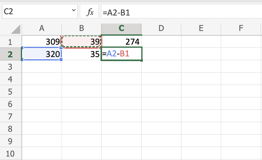
You got the result C2(281), right? Way to go!
Note: You can make formulas with all four arithmetic operations, such as addition (+), subtraction (-), multiplication (*) and division (/).
Here are some examples:
=2+4 gives you 6=4-2 gives you 2=2*4 gives you 8=2/4 gives you 0.5
In the next chapter you will learn about Ranges and how data can be moved in the Sheet.
Ranges
Range is an important part of Excel because it allows you to work with selections of cells.
There are four different operations for selection;
- Selecting a cell
- Selecting multiple cells
- Selecting a column
- Selecting a row
Before having a look at the different operations for selection, we will introduce the Name Box.
The Name Box
The Name Box shows you the reference of which cell or range you have selected. It can also be used to select cells or ranges by typing their values.
You will learn more about the Name Box later in this chapter.
Selecting a Cell
Cells are selected by clicking them with the left mouse button or by navigating to them with the keyboard arrows.
It is easiest to use the mouse to select cells.
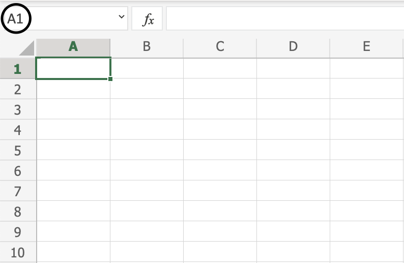
To select cell A1, click on it:
Selecting Multiple Cells
More than one cell can be selected by pressing and holding down CTRL or Command and left clicking the cells. Once finished with selecting, you can let go of CTRL or Command.
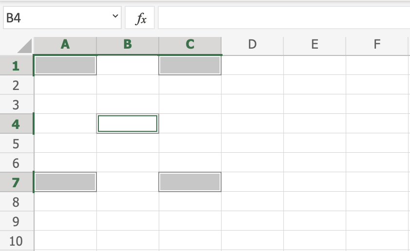
Lets try an example: Select the cells A1, A7, C1, C7 and B4.
Did it look like the picture below?
Selecting a Column
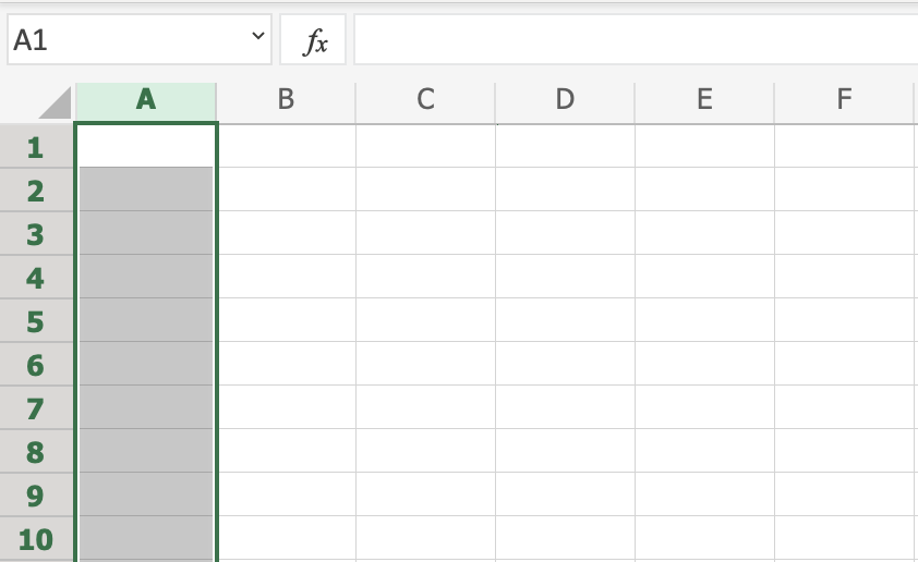
Columns are selected by left clicking it. This will select all cells in the sheet related to the column.
To select column A, click on the letter A in the column bar:
Selecting a Row
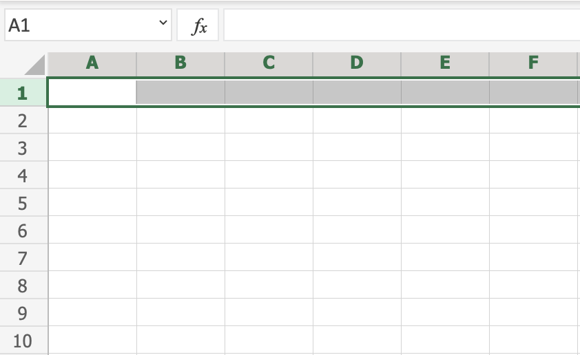
Rows are selected by left clicking it. This will select all the cells in the sheet related to that row.
To select row 1, click on its number in the row bar:
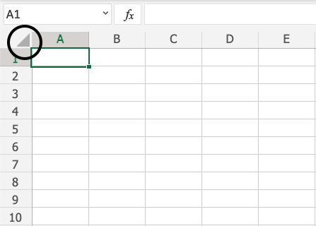
Selecting the Entire Sheet
The entire spreadsheet can be selected by clicking the triangle in the top-left corner of the spreadsheet: ![]()
Now, the whole spreadsheet is selected:
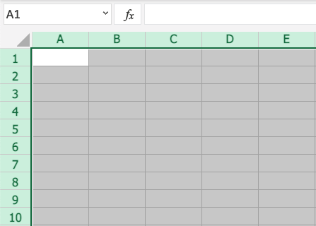
Note: You can also select the entire spreadsheet by pressing Ctrl+A for Windows, or Cmd+A for MacOS.
Selection of Ranges
Selection of cell ranges has many use areas and it is one of the most important concepts of Excel. Do not think too much about how it is used with values. You will learn about this in a later chapter. For now let's focus on how to select ranges.
There are two ways to select a range of cells
- Name Box
- Drag to mark a range.
The easiest way is drag and mark. Let's keep it simple and start there.
How to drag and mark a range, step-by-step:
- Select a cell
- Left click it and hold the mouse button down
- Move your mouse pointer over the range that you want selected. The range that is marked will turn grey.
- Let go of the mouse button when you have marked the range
Let's have a look at an example for how to mark the range A1:E10.
Note: You will learn about why the range is called A1:E10 after this example.
Select cell A1:
Press and hold A1 with the left mouse button. Move to the mouse pointer to mark the selection range. The grey area helps us to see the covered range.
Let go of the left mouse button when you have marked the range A1:E10:
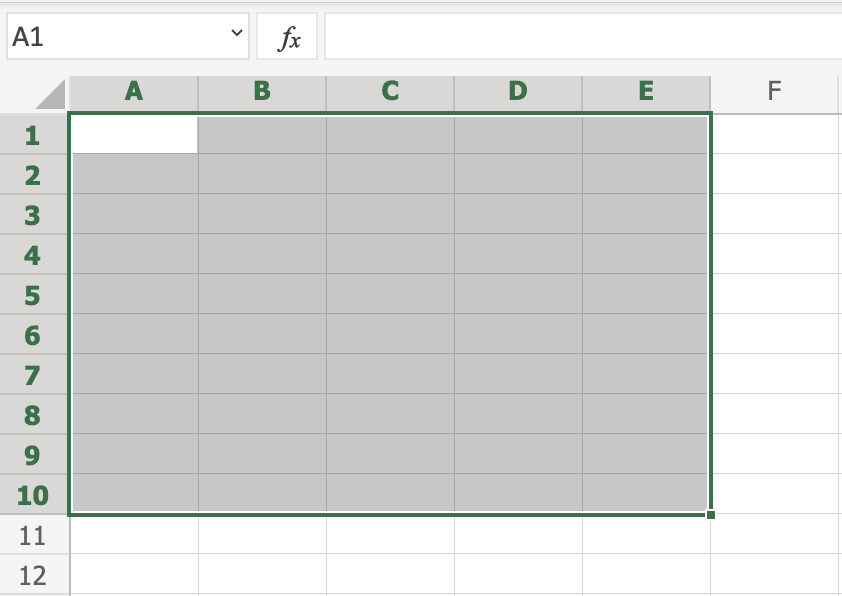
You have successfully selected the range A1:E10. Well done!
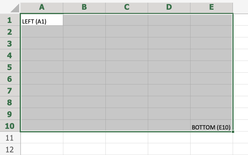
The second way to select a range is to enter the range values in the Name Box. The range is set by first entering the cell reference for the top left corner, then the bottom right corner. The range is made using those two as coordinates. That is why the cell range has the reference of two cells and the : in between.
Top left corner reference : Right bottom corner reference
The range shown in the picture has the value of A1:E10:
The best way for now is to use the drag and mark method as it is easier and more visual.
In the next chapter you will learn about filling and how this applies to the ranges that we have just learned.
Filling
Filling makes your life easier and is used to fill ranges with values, so that you do not have to type manual entries.
Filling can be used for:
- Copying
- Sequences
- Dates
- Functions (*)
For now, do not think of functions. We will cover that in a later chapter.
How To Fill
Filling is done by selecting a cell, clicking the fill icon and selecting the range using drag and mark while holding the left mouse button down.
The fill icon is found in the bottom right corner of the cell and has the icon of a small square. Once you hover over it your mouse pointer will change its icon to a thin cross.
Click the fill icon and hold down the left mouse button, drag and mark the range that you want to cover.
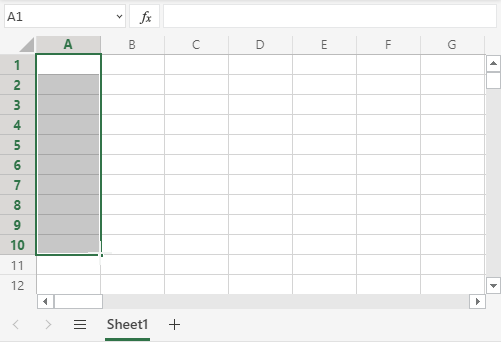
In this example, cell A1 was selected and the range A1:A10 was marked.
Now that we have learned how to fill. Let's look into how to copy with the fill function.
Fill Copies
Filling can be used for copying. It can be used for both numbers and words.
Let's have a look at numbers first.
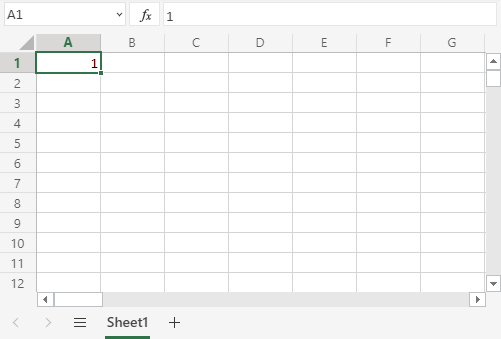
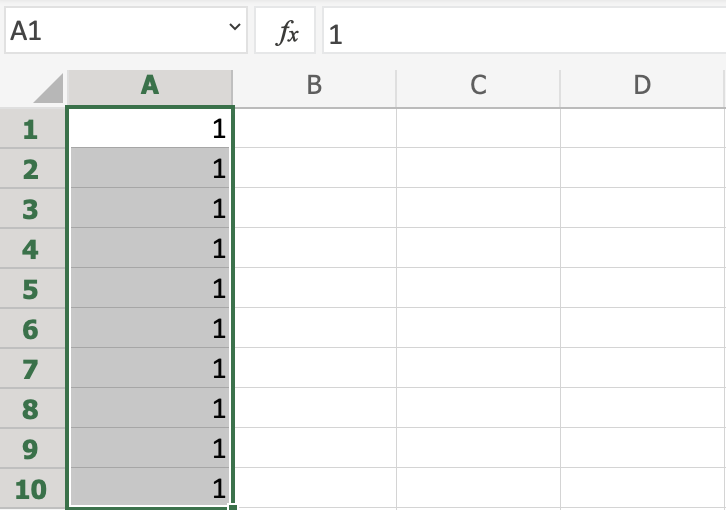
In this example we have typed the value A1(1):
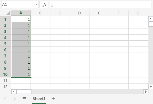
Filling the range A1:A10 creates ten copies of 1:
The same principle goes for text.
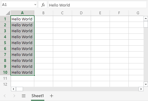
In this example we have typed A1(Hello World).
Filling the range A1:A10 creates ten copies of "Hello World":
Now you have learned how to fill and to use it for copying both numbers and words. Let's have a look at sequences.
Fill Sequences
Filling can be used to create sequences. A sequence is an order or a pattern. We can use the filling function to continue the order that has been set.
Sequences can for example be used on numbers and dates.
Let's start with learning how to count from 1 to 10.
This is different from the last example because this time we do not want to copy, but to count from 1 to 10.
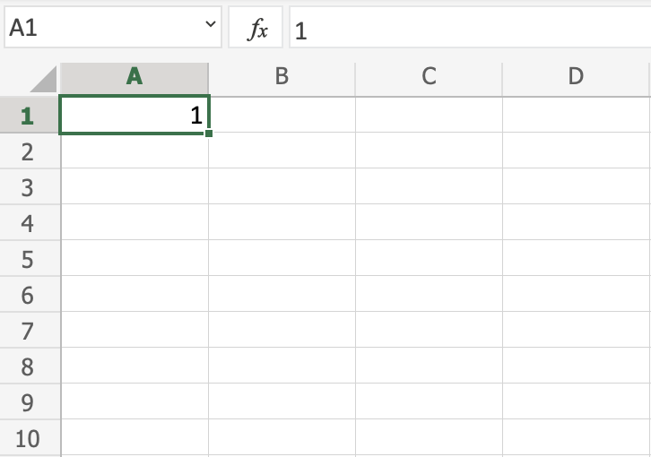
Start with typing A1(1):
First we will show an example which does not work, then we will do a working one. Ready?
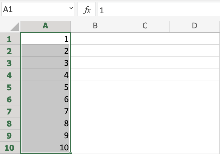
Lets type the value (1) into the cell A2, which is what we have in A1. Now we have the same values in both A1 and A2.
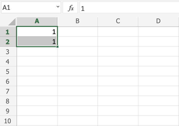
Let's use the fill function from A1:A10 to see what happens. Remember to mark both values before you fill the range.
What happened is that we got the same values as we did with copying. This is because the fill function assumes that we want to create copies as we had two of the same values in both the cells A1(1) and A2(1).
Change the value of A2(1) to A2(2). We now have two different values in the cells A1(1) and A2(2). Now, fill A1:A10 again. Remember to mark both the values (holding down shift) before you fill the range:
Congratulations! You have now counted from 1 to 10.
The fill function understands the pattern typed in the cells and continues it for us.
That is why it created copies when we had entered the value (1) in both cells, as it saw no pattern. When we entered (1) and (2) in the cells it was able to understand the pattern and that the next cell A3 should be (3).
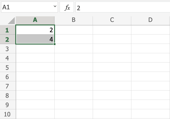
Let's create another sequence. Type A1(2) and A2(4):
Now, fill A1:A10:
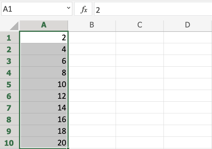
It counts from 2 to 20 in the range A1:A10.
This is because we created an order with A1(2) and A2(4).
Then it fills the next cells, A3(6), A4(8), A5(10) and so on. The fill function understands the pattern and helps us continue it.
Sequence of Dates
The fill function can also be used to fill dates.
Note: The date format depends on you regional language settings.
For example 14.03.2023 vs. 3/14/2023.
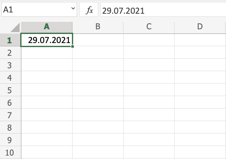
Test it by typing A1(29.07.2021):
And fill the range A1:A10:
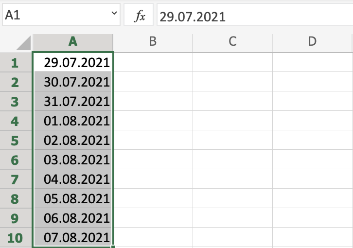
The fill function has filled 10 days from A1(29.07.2021) to A10(07.08.2021).
Note that it switched from July to August in cell A4. It knows the calendar and will count real dates.
Combining Words and Letters
Words and letters can also be combined.
Type A1(Hello 1) and A2(Hello 2):
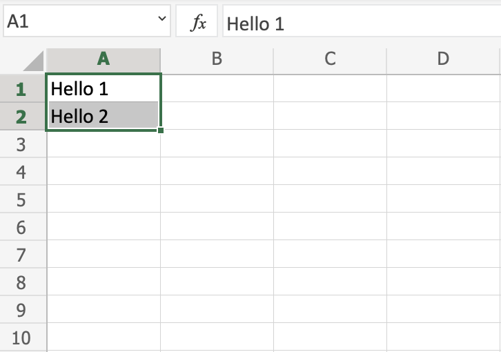
Next, fill A1:A10 to see what happens:
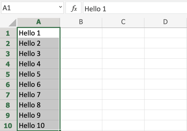
The result is that it counts from A1(Hello 1) to A10(Hello 10). Only the numbers have changed.
It recognised the pattern of the numbers and continued it for us. Words and numbers can be combined, as long as you use a recognizable pattern for the numbers.
Double Click to Fill
The fill function can be double clicked to complete formulas in a range:
Note: For the double click to work it has to see a recognizable pattern.
For example: by using headers, or with the formulas in the columns or rows next to the data.
Double Click to Fill Example
Let's use the Double click fill function to calculate the AttackB2:B20 + Defense C2:C20 for the Pokemons in the range D2:D20.
- Select
D2 - Type
=
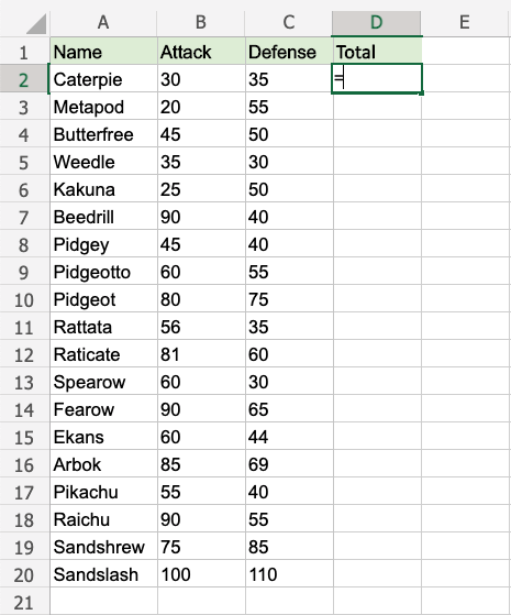
- Select
B2 - Type
+ - Select
C2
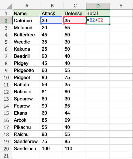
- Hit enter
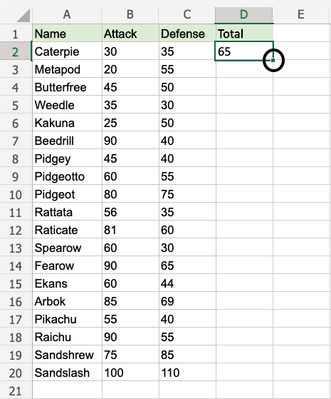
- Double click the fill function
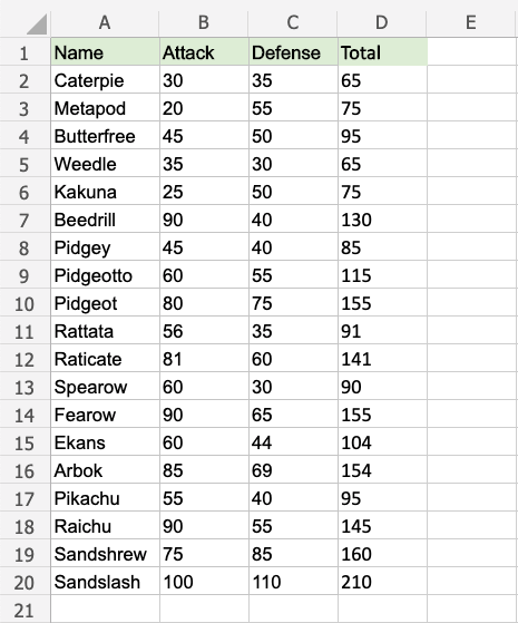
Way to go! The function understands the pattern and completes the calculation for D2:D20. Note that it stops when there is no more data to calculate, at row 20.
A Non-Working Example
Delete values in the range D1:D20
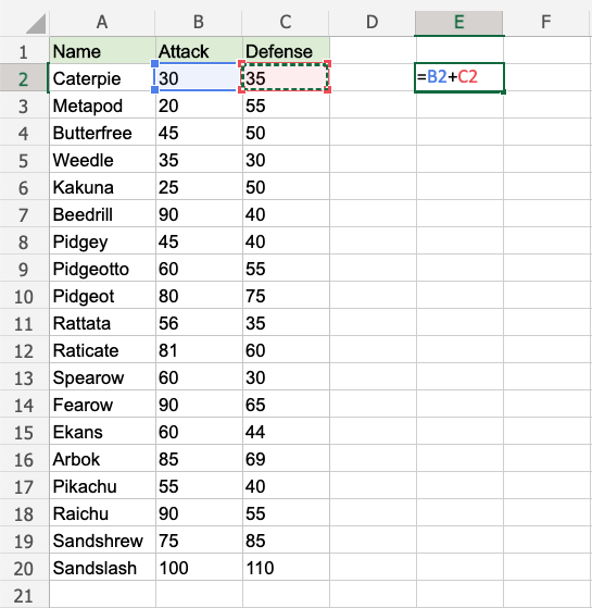
Enter the formula "=B2+C2" in E2
Note: There is no header for Columns D and E. There are blank cells in between.
Double click the fill function.
Waiting...
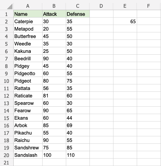
The fill function is just loading without filling the rows. It is not understanding the pattern.
Give it more clues.
Add a header to see what happens. Enter "Atk+def" in E1
Double click the fill function.
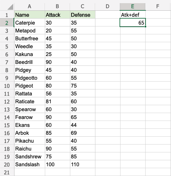
Loading... Still nothing...
One more header. Enter "Random" in D1
Double click the fill function.
Is the gap closed?
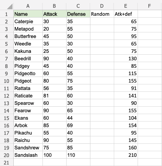
There we go! The function recognised the pattern and filled in the formulas for each row.
Adding headers helped the function to understand the relationship between the data.
Moving Cells
There are two ways to move cells: Drag and drop or by copy and paste.
Drag and Drop
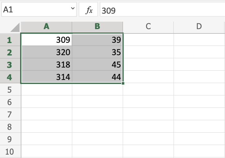
Let's start by typing or copying some values that we can work with:
Next, start by marking the area A1:B4:
You can drag and drop the range by pressing and holding the left mouse button on the border. The mouse cursor will change to the move symbol when you hover over the border.
Drag and drop it when you see the symbol.
Move the range to B2:C5 as shown in the picture:
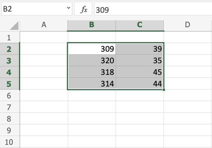
Great! Now you have created more space, so that we have room for more data.
Note: It is important to give context to the data, making the spreadsheet easy to understand. This can be done by adding text which explains the data.
Let's go ahead and give the data more context. Type or copy the following values:
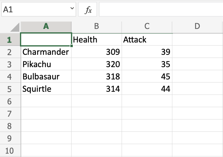
Yes, that is right, we are looking at Pokemons! Giving context to the data is always helpful.
Next, lets see how we can move data by using cut and paste.
Cut and Paste
Ranges can be moved by cutting and pasting values from one place to another.
Tip: You can cut using the hotkey CTRL+X and paste by CTRL+V. This saves you time.
Mark the range A1:C5
Right click the marked area, and click on the "Cut" command, which has scissors as its icon:
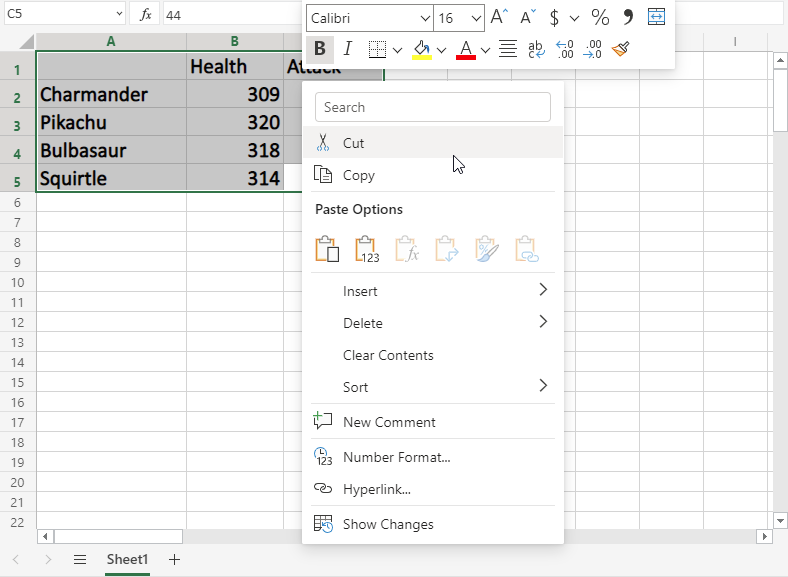
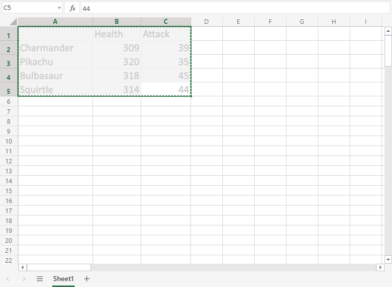
Cutting makes the range white-grey with dotted borders. This indicates that the range is cutted and ready for pasting.
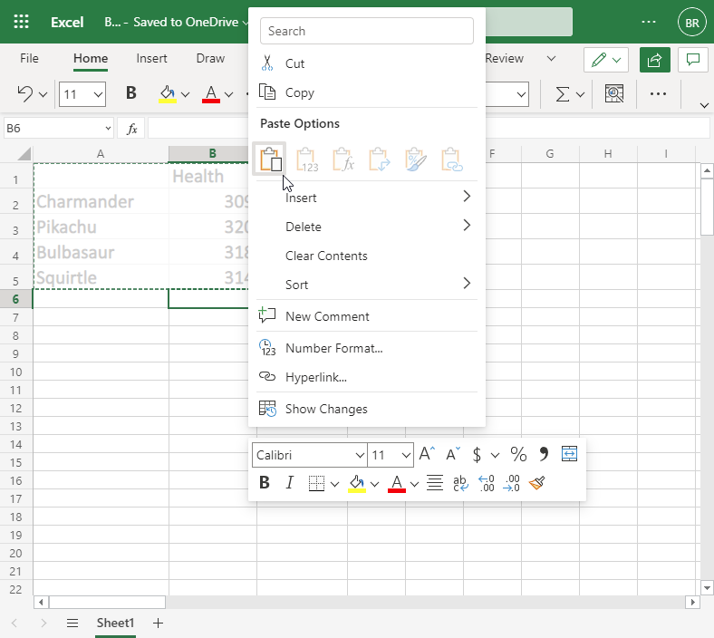
Right click the paste destination B6 and left click the paste icon.
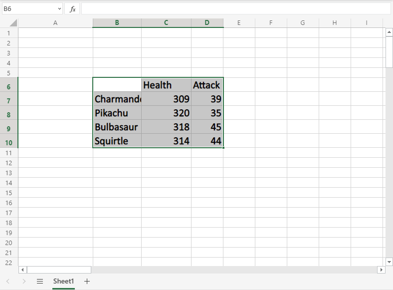
You have successfully cutted and pasted the range from A1:C5 to B6:D10.
Copy and paste
Copy and paste works in the same way as cut and paste. The difference is that it does not remove the original cells.
Let's copy the cells back from B6:D10 to A1:C5.
Tip: You can copy using the hotkey CTRL+C and paste by CTRL+V. This saves you time. Try it!
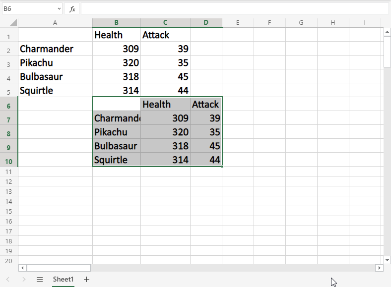
Mark the range B6:D10.
Right click the marked area, and click on the "Copy" command which has two papers as its icon.
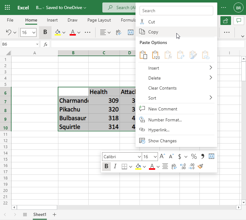
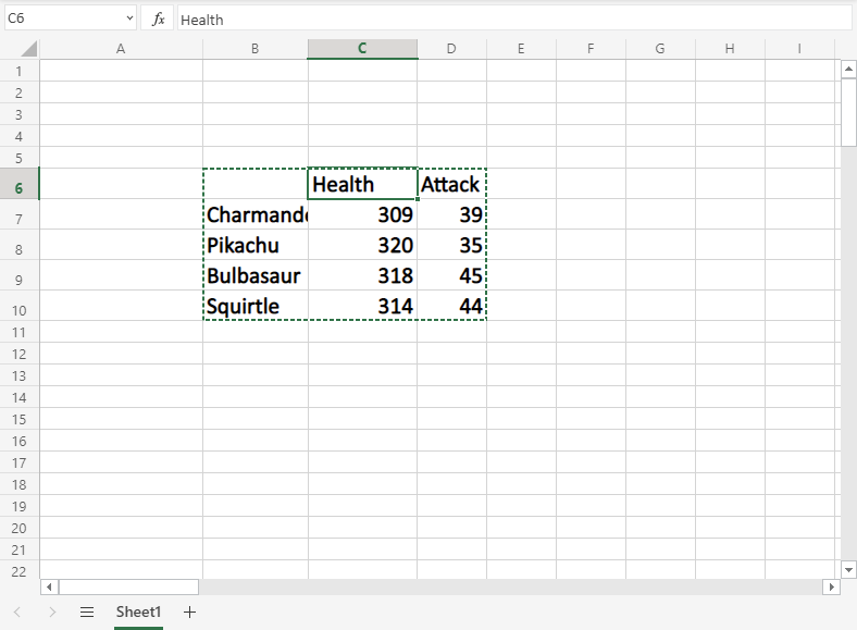
Copying gives the range a dotted green border. This indicates that the range is copied and ready for pasting.
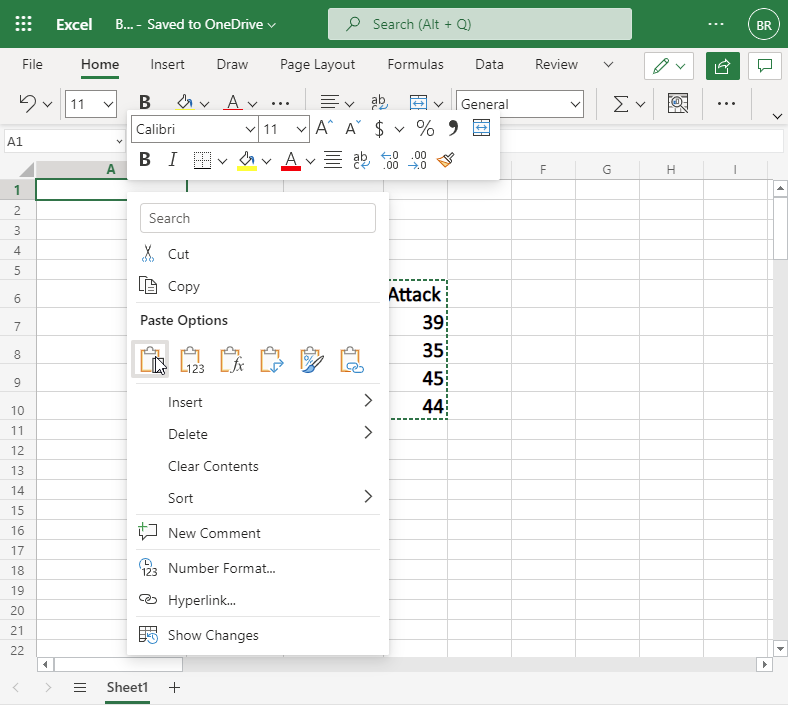
Right click the paste destination A1 and left click the paste icon:
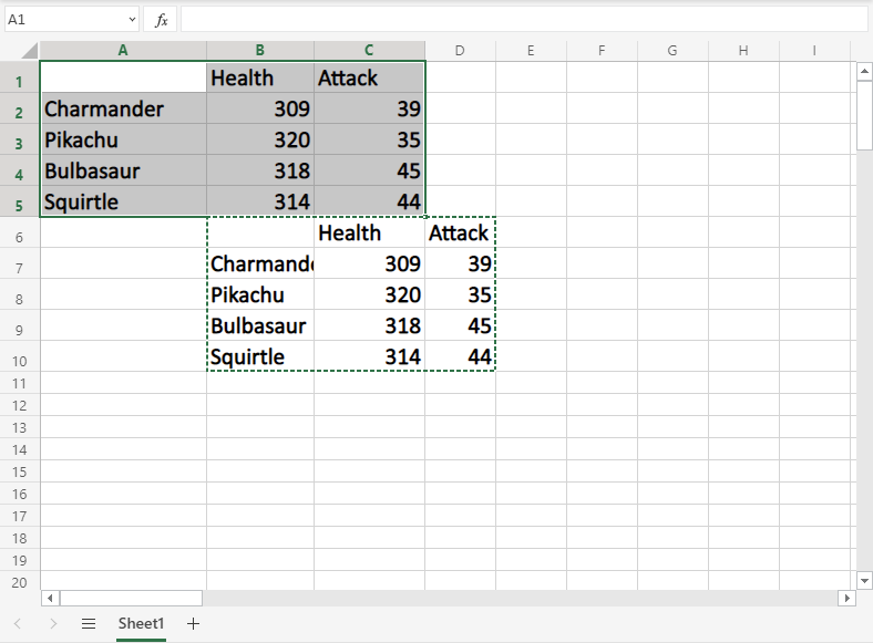
The difference between cutting and copying, is that cutting removes the originals, while copying leaves the originals.
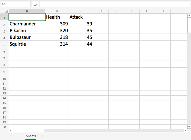
Next, let's delete the original data and keep the data in the A1:C5 range.
Delete Data
Select the original cells and remove them by pressing the "Delete" button on the keyboard:
Adding New Columns
Columns can be added and deleted. You access the menu by right clicking the column letter. New columns are added to the same place you clicked.
Let's try to create a new column B.
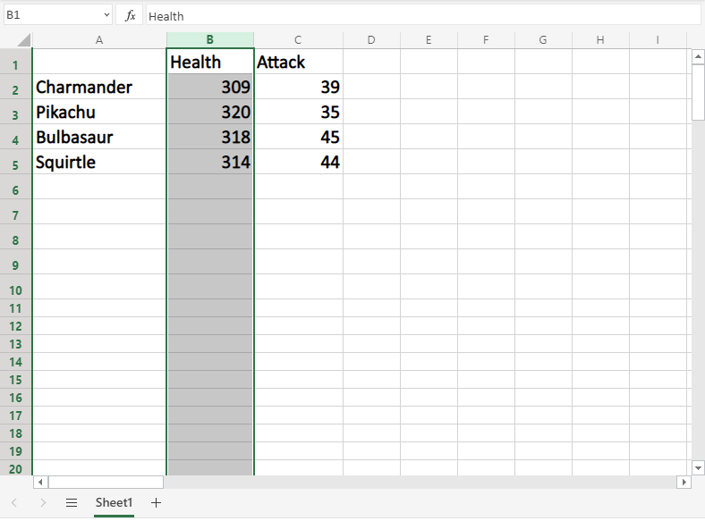
Right click on the column and select "Insert Columns":
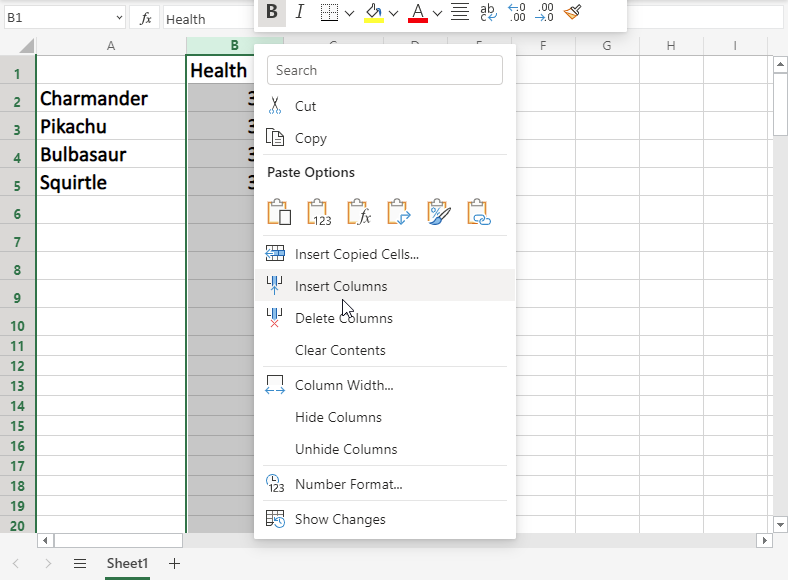
And a new column is created:

Next, we need to get some Pokemon trainers in there. Type or copy the following data in the new column B:
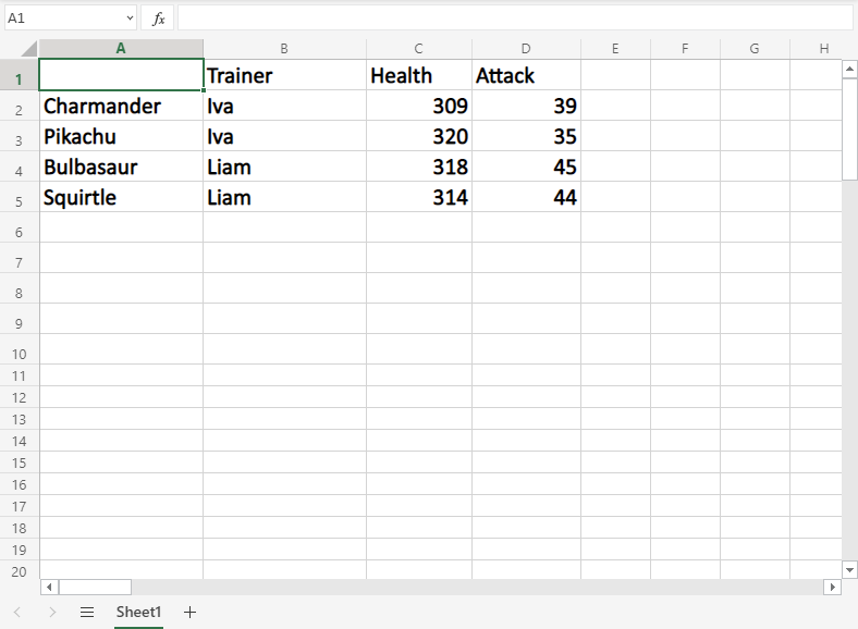
Adding New Rows
Rows can also be added and deleted. You access the menu by right clicking the row number. New rows are added to the same place you clicked.
Let's try to create a new row 4.
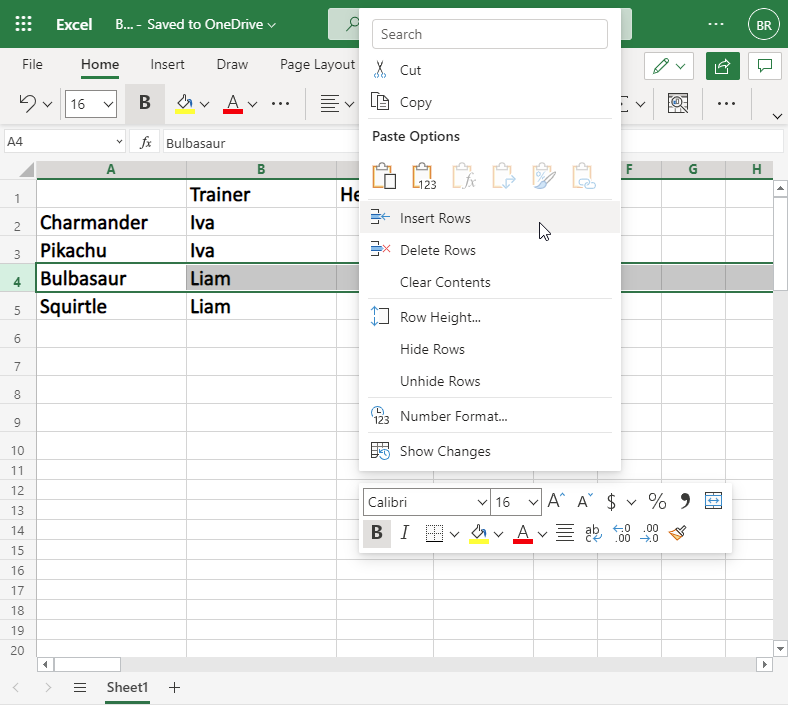
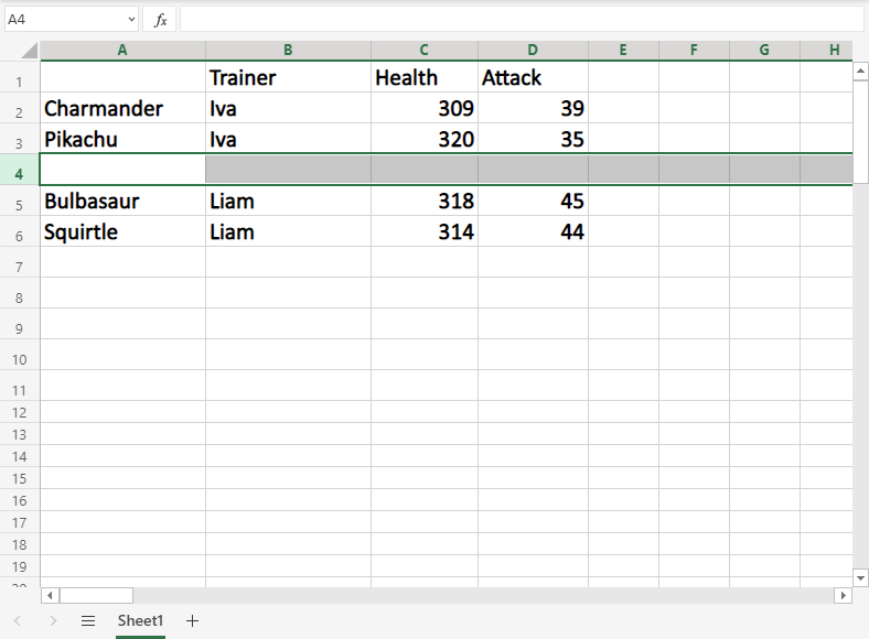
We forgot to add Iva's Pokemon, Marowak. Lets add his data to the new row 4, by typing or copying the following values:


0 Comments